Lab 5: Water Balance and Climate Classification
Background: In this lab we will be examining climate data at six sites across a transect of the eastern Columbia basin. These stations from west to east are: Connell, WA, La Crosse, WA, Pullman, WA, Moscow, ID and Elk River, ID shown here: http://alturl.com/c5ia3
Step 1: Download the 1971-2000 climate normals and station metadata
Place the following file on your MATLAB working directory on your computer: http://webpages.uidaho.edu/jabatzoglou/DATA/401/HW3DATA.mat
- Variable TMAX/TMIN are monthly average high and low temperature in degrees Celsius
- Variable PPT is monthly precipitation in mm
- Variable VS is the monthly average wind speed in meters per second.
- Variable RA is the monthly average insolation in W/m2.
- Variable NAME that tells you how stations are ordered.
Step 2: Download functions
Place these functions in your MATLAB directory on your computer.
Step 3: Calculate monthly potential evapotranspiration using the Penman-Montieth equation.
>> PET=monthlyPET_PM(RA,TMAX,TMIN,VS,LON,LAT,EL);
The output variable will be monthly PET in mm.
Step 4: Run the simple hydrologic model for each of your stations.
In MATLAB this can be done using a for loop
>>for i=1:5
>>[AET(i,:),DEF(i,:),RO(i,:)]=simplehydromodel(PPT(i,:),PET(i,:));
>>end
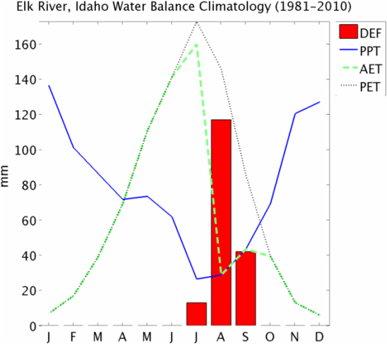
Step 5: Visualize your output
Plot monthly summaries of precipitation, PET, AET, DEF using the function waterbalancegraph2. For example, for the first station, ELK RIVER:
>>waterbalancegraph2(PPT(1,:),AET(1,:),DEF(1,:),PET(1,:))
>>title(‘Elk River, Idaho Water Balance Climatology (1981-2010)’,’fontsize’,20);
Place these functions in your MATLAB directory on your computer.
- http://webpages.uidaho.edu/jabatzoglou/DATA/401/monthlyPET_PM.m: used for calculating potential evapotranspiration
- http://webpages.uidaho.edu/jabatzoglou/DATA/401/simplehydromodel.m: used for running water balance model
- http://webpages.uidaho.edu/jabatzoglou/MATLAB/waterbalancegraph2.m : used for visualizing data
Step 3: Calculate monthly potential evapotranspiration using the Penman-Montieth equation.
>> PET=monthlyPET_PM(RA,TMAX,TMIN,VS,LON,LAT,EL);
The output variable will be monthly PET in mm.
Step 4: Run the simple hydrologic model for each of your stations.
In MATLAB this can be done using a for loop
>>for i=1:5
>>[AET(i,:),DEF(i,:),RO(i,:)]=simplehydromodel(PPT(i,:),PET(i,:));
>>end
Step 5: Visualize your output
Plot monthly summaries of precipitation, PET, AET, DEF using the function waterbalancegraph2. For example, for the first station, ELK RIVER:
>>waterbalancegraph2(PPT(1,:),AET(1,:),DEF(1,:),PET(1,:))
>>title(‘Elk River, Idaho Water Balance Climatology (1981-2010)’,’fontsize’,20);